Cross Correlation
The general form of the cross correlation with integration: \begin{equation} {\displaystyle (f\star g)(\tau )\ = \int _{-\infty }^{\infty }{{f^{\star}(t)}}g(t+\tau )\,dt} \end{equation} This can be written in discrete form as: \begin{equation} {\displaystyle (f\star g)[n]\ = \sum _{m=-\infty }^{\infty }{{f^{\star}[m]}}g[m+n]} \end{equation}
[1]:
from matplotlib import pylab
from matplotlib import pyplot as plt
pylab.rcParams['savefig.dpi'] = 300
import numpy as np
[2]:
from gps_helper.prn import PRN
from sk_dsp_comm import sigsys as ss
from sk_dsp_comm import digitalcom as dc
from caf_verilog.quantizer import quantize
Test Signals
[3]:
prn = PRN(10)
prn2 = PRN(20)
fs = 625e3
Ns = fs / 125e3
prn_seq = prn.prn_seq()
prn_seq2 = prn2.prn_seq()
prn_seq,b = ss.nrz_bits2(np.array(prn_seq), Ns)
prn_seq2,b2 = ss.nrz_bits2(np.array(prn_seq2), Ns)
[4]:
Px,f = plt.psd(prn_seq, 2**12, Fs=fs)
plt.plot(f, 10*np.log10(Px))
[4]:
[<matplotlib.lines.Line2D at 0x7f229e1c9b40>]

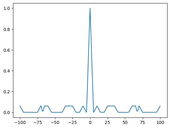
Autocorrelation
[5]:
r, lags = dc.xcorr(prn_seq, prn_seq, 100)
plt.plot(lags, abs(r)) # r -> abs
[5]:
[<matplotlib.lines.Line2D at 0x7f229c07f250>]
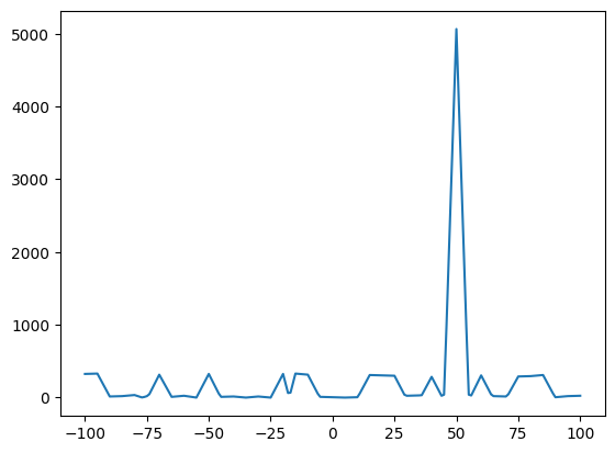
Time Shifted Signals
[6]:
r, lags = dc.xcorr(np.roll(prn_seq, 50), prn_seq, 100)
plt.plot(lags, abs(r))
[6]:
[<matplotlib.lines.Line2D at 0x7f229c11a380>]

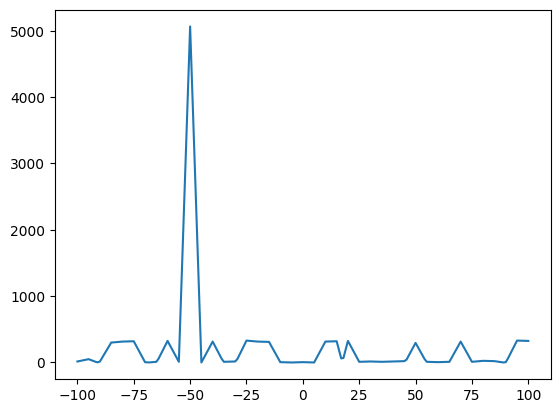
[7]:
r, lags = dc.xcorr(np.roll(prn_seq, -50), prn_seq, 100)
plt.plot(lags, abs(r))
[7]:
[<matplotlib.lines.Line2D at 0x7f229bfa18a0>]

No Correlation
[8]:
r_nc, lags_nc = dc.xcorr(prn_seq, prn_seq2, 100)
plt.plot(lags_nc, abs(r_nc))
plt.ylim([0, 1])
[8]:
(0.0, 1.0)

Calculation Space Visualization
[9]:
from caf_verilog.xcorr import size_visualization
size_visualization(prn_seq[:10], prn_seq[:10], 5)
n: -5 [(5, 0), (6, 1), (7, 2), (8, 3), (9, 4)]
n: -4 [(4, 0), (5, 1), (6, 2), (7, 3), (8, 4), (9, 5)]
n: -3 [(3, 0), (4, 1), (5, 2), (6, 3), (7, 4), (8, 5), (9, 6)]
n: -2 [(2, 0), (3, 1), (4, 2), (5, 3), (6, 4), (7, 5), (8, 6), (9, 7)]
n: -1 [(1, 0), (2, 1), (3, 2), (4, 3), (5, 4), (6, 5), (7, 6), (8, 7), (9, 8)]
n:  0 [(0, 0), (1, 1), (2, 2), (3, 3), (4, 4), (5, 5), (6, 6), (7, 7), (8, 8), (9, 9)]
n:  1 [(0, 1), (1, 2), (2, 3), (3, 4), (4, 5), (5, 6), (6, 7), (7, 8), (8, 9)]
n:  2 [(0, 2), (1, 3), (2, 4), (3, 5), (4, 6), (5, 7), (6, 8), (7, 9)]
n:  3 [(0, 3), (1, 4), (2, 5), (3, 6), (4, 7), (5, 8), (6, 9)]
n:  4 [(0, 4), (1, 5), (2, 6), (3, 7), (4, 8), (5, 9)]
n:  5 [(0, 5), (1, 6), (2, 7), (3, 8), (4, 9)]
Simple Cross Correlation
[10]:
from caf_verilog.xcorr import simple_xcorr
r, lags = simple_xcorr(prn_seq, prn_seq, 100)
plt.plot(lags, r)
[10]:
[<matplotlib.lines.Line2D at 0x7f229bd4f7f0>]

Time Shifted Signals
[11]:
r, lags = simple_xcorr(prn_seq, np.roll(prn_seq, 50), 100)
plt.plot(lags, abs(np.array(r)))
[11]:
[<matplotlib.lines.Line2D at 0x7f229bdd6b30>]
[12]:
r, lags = simple_xcorr(prn_seq, np.roll(prn_seq, -50), 100)
plt.plot(lags, abs(np.array(r)))
[12]:
[<matplotlib.lines.Line2D at 0x7f229bc65f60>]
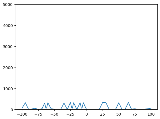
No Correlation
[13]:
r, lags = simple_xcorr(prn_seq, prn_seq2, 100)
plt.plot(lags, abs(np.array(r)))
plt.ylim([0, 5000])
[13]:
(0.0, 5000.0)
Dot Product Method
To ensure the integration time is filled, the secondary or received signal must be twice the length of the reference signal.
[14]:
from caf_verilog.sim_helper import sim_shift
center = 300
corr_length = 250
shift = 25
ref, rec = sim_shift(prn_seq, center, corr_length, shift=shift, padding=True)
ref = np.array(ref)
rec = np.array(rec)
[15]:
f, axarr = plt.subplots(2, sharex=True, gridspec_kw={'hspace': 0})
axarr[0].plot(ref.real)
axarr[1].plot(rec.real)
plt.xlabel("Sample Number")
plt.savefig('prn_seq.png')

[16]:
from caf_verilog.xcorr import dot_xcorr
ref = np.array(ref)
rec = np.array(rec)
rr = dot_xcorr(ref, rec)
rr = np.array(rr)
[17]:
rxy, lags = dc.xcorr(ref, rec, corr_length)
plt.plot(lags, abs(rxy))
plt.xlabel("Center Offset (Samples)")
plt.grid();
plt.savefig('xcorr.png')

[18]:
np.argmax(rxy) - corr_length
[18]:
25
[19]:
ref, rec = sim_shift(prn_seq, center, corr_length, shift=shift)
ref = np.array(ref)
rec = np.array(rec)
rr = dot_xcorr(ref, rec)
rr = np.array(rr)
[20]:
fig, axs = plt.subplots(2, sharey=True)
axs[0].plot(abs(rr))
axs[0].grid(True)
axs[1].plot(abs(rr))
axs[1].set_xlim([80, 120])
axs[1].set_xlabel('Inverse Center Offset (Samples)')
axs[1].grid(True)
fig.savefig('xcorr_250.png')
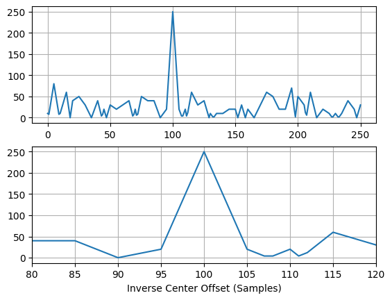
[21]:
(corr_length / 2) - np.argmax(rr)
[21]:
25.0
[22]:
from caf_verilog.xcorr import XCorr
xc = XCorr(ref, rec, output_dir='.')
[23]:
xc.gen_tb()